

Store Sales & Calculations
Revenue and Calc translate monthly visits, conversion, 3.5 units per transaction, merchandise shares, and unit prices into five category sales forecasts.


The Fabric Store Financial Model is an Excel financial planning template for an independent fabric and sewing-supplies retailer. It links store traffic, purchase conversion, merchandise units, category prices, inventory costs, staffing, and overhead to monthly projections and a five-year operating forecast.
The illustrated case models a leased 2,000-square-foot store in a secondary Midwestern US market, launching January 31, 2026. It covers in-store fabric, batting, and notions sales from 2026 through 2030; sewing machines, classes, alterations, and online sales are outside this case.
The workbook connects store-specific planning assumptions to financial statements, funding schedules, and analytical reports.
Revenue and Calc translate monthly visits, conversion, 3.5 units per transaction, merchandise shares, and unit prices into five category sales forecasts.
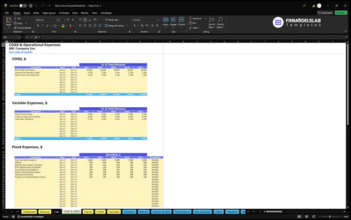
COGS & OPEX and Payroll separate inventory-related expenses, transaction-variable charges, store overhead, and role-based salary costs.
CAPEX, CapTable, Debt, and Sources & Uses organize store fixtures, opening contributions, optional borrowing assumptions, and related cash movements.
IS, CF, BS, Dashboard, Summary, Scenarios, Returns, Valuation, Charts, and Checks support financial review and model reconciliations.
The revenue forecast begins with customer demand rather than shelf capacity: visits turn into purchases, selling units, and category-level sales.
Each active month uses store visits × purchase conversion × 3.5 units per transaction. One fabric or batting unit represents one yard; one notions unit represents one pack or item. Those units are allocated once among five mutually exclusive merchandise categories.
The model assigns 40% of units to quilting cotton, 20% to apparel fabric, 10% to home decor fabric, 10% to batting and interfacing, and the remaining 20% to sewing notions. Corresponding estimated net prices are $12, $16, $25, $18, and $5 per selling unit.
The Revenue Forecast connects traffic, purchase conversion, units per transaction, category allocation, and net selling prices. Monthly calculations flow into annual sales by merchandise category, allowing a store owner to test changes in demand or product mix.
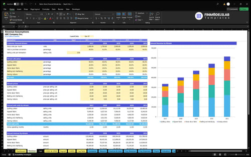
1,500 visits × 40% conversion × 3.5 units × $13.30 weighted unit price = $27,930 in monthly revenue.
The same price and merchandise shares apply across the illustrated years; demand assumptions drive the growth. Monthly visits rise from 1,500 in 2026 to 2,500 in 2030, while conversion improves from 40% to 44%. No separate seasonal pattern or additional sales channel is assumed.
Costs are separated into merchandise COGS, revenue-linked selling expenses, monthly fixed overhead, and salaries so that each expense is counted once.
The illustration estimates merchandise purchases at 50% of revenue, inbound freight at 2.5%, and shrink or cutting losses at 1.5%. Together they create a 54% COGS assumption. Payment processing, packaging, and local marketing add another 6% of revenue as variable expenses.
Fixed costs cover rent, utilities, insurance, POS connectivity, accounting, repairs, cleaning, security, and administration. The estimated $3,000 monthly rent is part of the $53,640 annual fixed-cost total; it is not charged a second time.
The COGS and Operating Expenses forecast separates direct merchandise costs from transaction-related spending and recurring retail overhead. It helps show how a different sales level or merchandise cost percentage changes contribution margin and operating EBITDA.
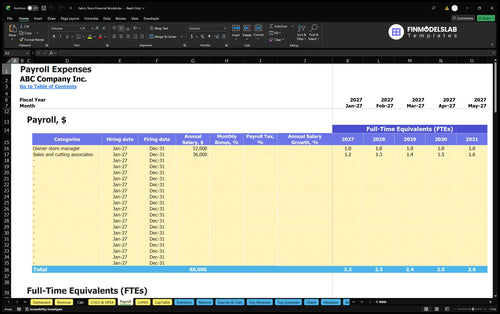
Payroll uses one full-time owner-manager at an estimated $52,000 annual base salary plus sales and cutting associates at $36,000 per annual-average FTE. Associate staffing grows from 1.2 FTE in 2026 to 1.6 FTE in 2030, with salary expense kept separate from COGS and other overhead.
The Payroll Forecast details staffing by role, FTE assumptions, hiring schedules, and base compensation. In this case, planned annual salary expense rises from $95,200 in 2026 to $109,600 in 2030 as associate coverage expands.
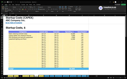
Startup investment and working-capital requirements are modeled separately from the operating expenses used to calculate EBITDA.
Estimated opening assets include $16,000 for fabric shelving and bolt racks, $6,000 for cutting tables and checkout fixtures, $4,000 for POS and security equipment, and $12,000 for leasehold lighting and fitout. That is $38,000 of identified startup assets, before other opening cash needs.
Separate items cover a refundable premises deposit, preopening branding, permits and professional setup, and preopening staff pay. Inventory is included in opening net working capital rather than counted again as a separate startup cash purchase.
The Capital Expenditure Plan schedules retail fixtures, equipment, and leasehold improvements and tracks depreciable spending where applicable. This distinguishes investments needed to open the store from merchandise expenses recognized in the operating forecast.
The illustrative plan uses zero accounts-receivable days, 15 accounts-payable days, and 90 inventory days. Estimated initial owner funding is $177,173, including a $87,484 three-month reserve based on first-year monthly operating outflows. No loan or grant is assumed in this example.
The Sources and Uses of Funds report organizes owner contributions, potential financing sources, store setup spending, operating cash payments, and cash retained. Use it to evaluate how an opening funding plan differs from the annual EBITDA forecast.

The estimated case moves from a first-year operating loss to positive EBITDA as retail traffic and conversion increase.
| Year | Revenue | Operating Expenses | EBITDA |
|---|---|---|---|
| 2026 | $335,160 | $349,936 | -$14,776 |
| 2027 | $400,796 | $392,917 | $7,878 |
| 2028 | $469,224 | $437,574 | $31,650 |
| 2029 | $540,446 | $483,907 | $56,538 |
| 2030 | $614,460 | $531,916 | $82,544 |
Illustrative estimates, not observed store results. Amounts rounded to whole dollars; source calculations retain decimals.
Revenue rises from $335,160 in 2026 to $614,460 in 2030. Operating expenses include the direct costs, selling-variable costs, recurring overhead, and payroll outlined above; projected EBITDA changes from a loss of $14,776 to a positive $82,544.
EBITDA is operating earnings before depreciation, interest, and taxes, not net profit or cash available for distribution. The model includes income statement, balance sheet, and cash flow reports, but the supplied numerical illustration establishes operating results only through EBITDA.
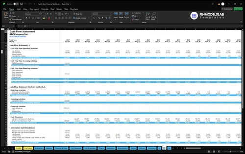
The Cash Flow Forecast presents operating, investing, and financing cash movements and reconciles opening to closing cash. It is the relevant report for examining inventory purchases, retail receipts, fixture spending, and owner funding without treating EBITDA as cash flow.
The selected launch date is January 31, 2026. All sales streams are zero before launch, and the launch month is treated as a full normal selling month; annual revenue totals are the sum of monthly results.
The Returns and scenario reports provide separate views of operating thresholds, funding recovery, and the effects of changed assumptions.
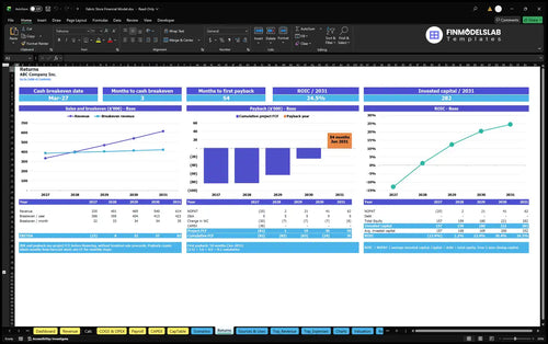
The Returns worksheet distinguishes sales break-even from cash break-even, cumulative investment payback, and annual return on invested capital. These are different tests: covering operating costs does not automatically mean cash has been recovered or invested capital has earned a particular return.
The valuation and financial statement reports can support additional review, including discounted cash flow sensitivity and financing impact. The source example provides no verified break-even month, payback period, ROIC, or valuation, so none is asserted here.
The Returns analysis compares revenue with sales break-even needs and examines project cash flow, cumulative payback, and annual ROIC. For a fabric retailer, it separates an acceptable trading margin from recovery of fitout and opening funding.
Dashboard scenario controls let users select Low, Base, or High multipliers for revenue, COGS, variable expenses, fixed expenses, and payroll. Compare their results to see whether a slower visitor ramp, higher buying costs, or extra staffing could erode the operating margin.
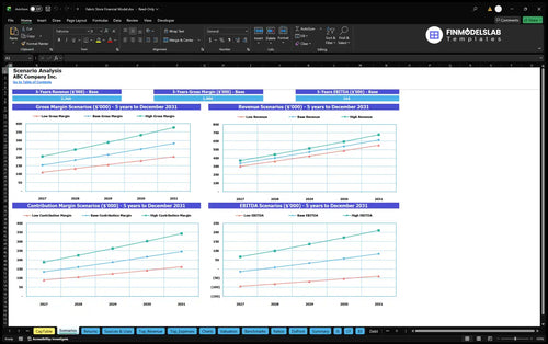
The Financial Scenario Analysis report compares Low, Base, and High cases for revenue, gross margin, contribution margin, and EBITDA. Its comparative output helps identify which operating assumptions need the most attention before signing a lease or setting staffing levels.
These answers clarify the template’s revenue calculations, reporting scope, and funding assumptions.
Monthly store visits, purchase conversion, 3.5 selling units per transaction, merchandise category shares, and estimated selling prices determine the in-store revenue forecast.
One fabric or batting unit is one yard; one sewing-notions unit is one pack or item. Each selling unit is assigned to one category.
Yes. The Payroll worksheet supports FTE planning, salary assumptions, and hiring schedules; the example starts with a manager and sales/cutting associates.
It includes working-capital controls for inventory, receivables, and payables. The sample assumptions are 90, zero, and 15 days, respectively.
No. That projected EBITDA is before depreciation, interest, and taxes and does not establish accounting net profit or free cash flow.
No. It assumes estimated owner funding of $177,173, while the workbook separately provides debt controls for user-defined financing scenarios.
Yes. The workbook has Cash Flow, Sources & Uses, and Returns reports, but the supplied illustration does not establish specific payback or cash-sufficiency results.
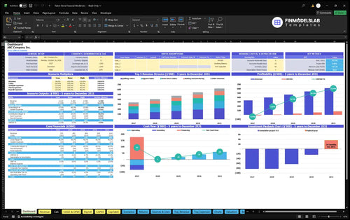
KPIs, forecasts, and cash flow at a glance.
Key assumptions and calculations driving revenue forecasts.
Funding sources, spending, and closing cash.
Cash break-even, payback, and ROIC.
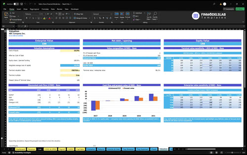
DCF valuation and sensitivity analysis.
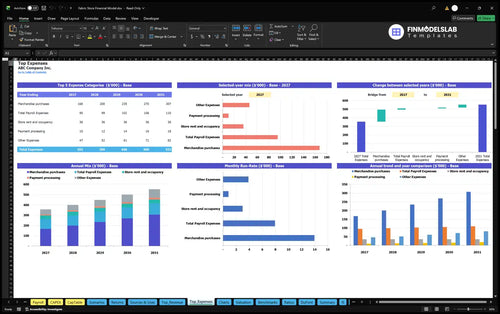
Largest costs and spending trends.
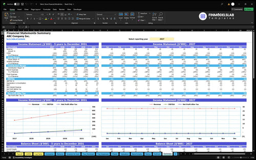
Annual and monthly financial performance.
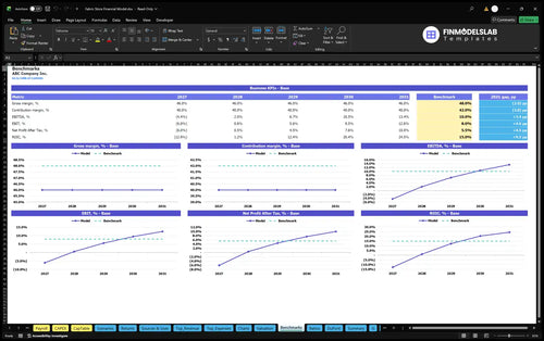
Compare margins and returns to benchmarks.

Building the model from scratch would’ve taken me days, but this template cut the setup down to an afternoon. I saved at least 12 hours and had my numbers ready to share much faster.
The pricing, cost, and growth inputs finally sit in one place instead of scattered across tabs. I was able to clean up my assumptions in under an hour and explain them without second-guessing.
I wasn’t sure what investors wanted to see, but this model gave me the right structure right away. It helped me walk into a meeting with a clear five-year view and book a follow-up the same week.