

Revenue & Calc
Edit launch timing, daily transactions, operating days, items per transaction, department mix, and realized prices. Monthly calculations allocate sold units to the five departments and consolidate sales.


The Grocery Store Financial Model is an Excel template for building financial projections from checkout transactions, items purchased, departmental prices, operating expenses, and staffing. Its illustrative operating case covers 2026 through 2030 and shows how these assumptions determine revenue and EBITDA.
The case represents an approximately 6,000-square-foot independent US neighborhood grocery store with staffed checkout and five merchandise departments. All selected assumptions are Estimated planning inputs; the store has no pharmacy, fuel, alcohol, or prepared-meal operation.
Connected inputs and reports help evaluate how store demand, merchandise costs, staffing, and opening investment affect the plan.
Edit launch timing, daily transactions, operating days, items per transaction, department mix, and realized prices. Monthly calculations allocate sold units to the five departments and consolidate sales.
Set merchandise costs, shrink, transaction-related expenses, monthly overhead, and role-based staffing. Separate payroll calculations keep base salaries distinct from other operating costs.
Select Low, Base, or High assumptions using separate multipliers for revenue, COGS, variable expenses, fixed expenses, and payroll. Compare their effects on margins and EBITDA.
Review financial statements and the combined reporting view for profitability, inventory, payables, and financing. The supplied grocery case establishes numeric operating results through EBITDA only.
One transaction forecast determines all sold items, which are allocated once across the five merchandise departments.
Daily transactions increase from 200 in 2026 to 380 in 2030, with 30 operating days per month and nine items per transaction throughout. Sales activate in the launch month, January 2026; preceding months have zero sales.
Dry Grocery receives 45% of item units, Fresh Produce 20%, Dairy and Frozen 20%, Meat and Seafood 10%, and Household Supplies 5%. These are unit shares; each department's realized price determines its dollar sales.
The Revenue Forecast connects operating drivers, sold-item volume, departmental prices, and revenue. Adjust transaction growth or pricing to evaluate sales changes; this demand-based case has no separate capacity ceiling.
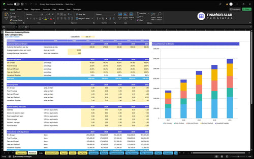
200 daily transactions × 30 days × 9 items × $4.325 weighted item price × 12 months = $2,802,600 annual revenue.
The weighted item price uses the department mix above and 2026 prices of $3.50, $3.25, $4.25, $9.00, and $7.00, respectively. Annual price assumptions and transaction growth both contribute to the illustrated revenue increase.
Revenue-based expenses scale with sales, while fixed overhead and staffing follow their own assumptions.
The COGS & Operating Expense Forecast separates direct merchandise costs, variable expenses, and fixed overhead. Landed merchandise sold is estimated at 70% of revenue, with inventory shrink and spoilage adding 2.5%.
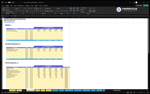
Merchant processing is 2.3% of revenue; checkout consumables and sales-linked loyalty each add 0.3%. Together, COGS and variable expenses leave 24.6% of revenue to cover fixed overhead and payroll before EBITDA.
Fixed expenses include occupancy, utilities, refrigeration service, insurance, systems, marketing, and other store overhead. Annual fixed costs rise from $351,600 to $393,792; monthly rent and occupancy increase from $15,000 to $16,800, with 12 paid months annually.
The Payroll Forecast calculates personnel costs from staffing FTE and compensation by role. Cashiers, receiving staff, fresh-department staff, management, and administration total 14.5 annual-average FTE in 2026 and 20.6 in 2030, with annual base payroll of $572,000 and $798,000.
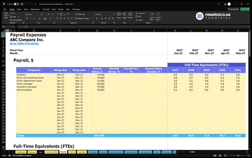
Base salaries are counted once through Payroll and excluded from the other cost categories. Employer taxes, employee benefits, and owner personal taxes are excluded from this illustrative case, so staffing decisions should account for those scope limits.
Startup assets, preopening cash, working capital, and owner contributions are distinct from the annual operating expense forecast.
The Capital Expenditure Plan schedules asset purchases and depreciation. Selected opening assets include $145,000 for refrigeration, $45,000 for shelving, $180,000 for leasehold and electrical fitout, and $26,000 for checkout hardware, alongside other equipment.

Separate preopening cash covers the lease deposit, permits and setup, marketing, training pay, rent, and utilities. Working-capital controls assume zero receivable days, 11 payable days, and 21 inventory days, connecting supplier terms and stockholding to funding needs.
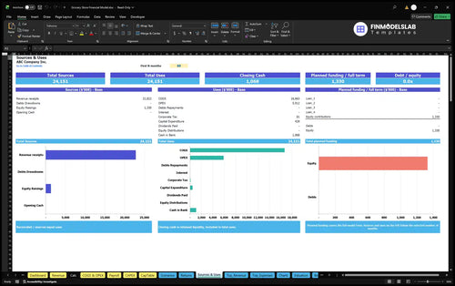
Sources and Uses of Funds reconciles funding sources and cash allocation over a selected period. Estimated initial owner funding is $1,329,503, based on assets, separate prelaunch cash, opening material net working capital, and three months of first-year cash OPEX including base payroll once.
The supplied case reaches positive annual EBITDA in 2028 as sales growth exceeds the increase in operating costs.
| Year | Revenue | Operating Expenses | EBITDA |
|---|---|---|---|
| 2026 | $2,802,600 | $3,036,760 | -$234,160 |
| 2027 | $3,901,608 | $3,931,460 | -$29,852 |
| 2028 | $4,764,096 | $4,651,824 | $112,272 |
| 2029 | $5,363,820 | $5,170,064 | $193,756 |
| 2030 | $5,989,788 | $5,708,092 | $281,696 |
Illustrative projections, not industry averages; independently rounded whole-dollar figures may differ slightly.
Operating expenses combine COGS, variable expenses, fixed overhead, and payroll. Positive annual EBITDA does not establish net profit, monthly cash break-even, or investment recovery; the forecast provides no numeric conclusions for those measures.
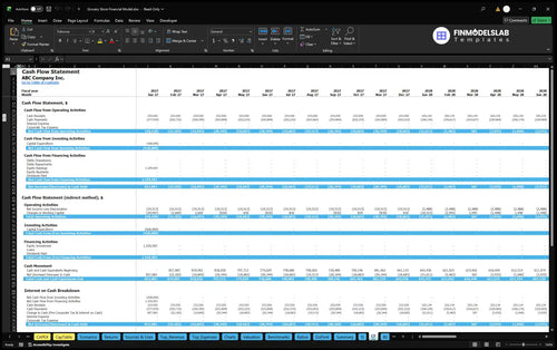
The Cash Flow Forecast separates operating, investing, and financing cash movements and reconciles opening to closing cash. Use it to assess inventory funding, supplier payments, capital spending, and financing timing after reviewing the relevant workbook inputs.
Returns and financing controls support separate evaluations of operating coverage, liquidity timing, capital recovery, and investment performance.
Dashboard Debt Controls feed financing schedules for facility amounts, dates, rates, terms, and repayment structures. Enter contemplated borrowing alongside owner contributions to examine funding alternatives; the supplied case does not establish a debt facility or loan eligibility.
Return on Invested Capital Analysis combines sales break-even, cash break-even, investment payback, and annual ROIC in the Returns report. It helps compare cost coverage and investment performance using the completed model's supporting calculations.
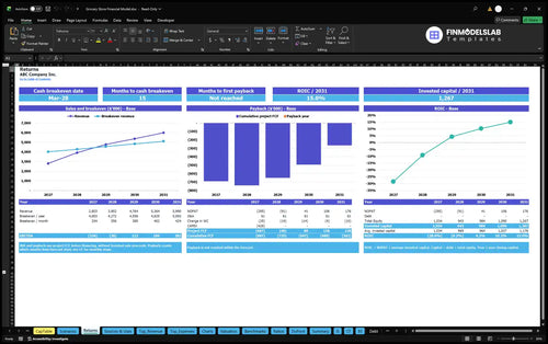
Sales break-even evaluates revenue needed to cover operating costs; cash break-even considers cash timing. Investment payback assesses recovery through cumulative project cash flow, while annual ROIC measures returns against invested capital; none can be determined from EBITDA alone.
The template fits an independent neighborhood grocery plan with department-level merchandise sales and salaried store staffing.
Replace the generic metropolitan or suburban lease assumptions with your proposed property costs, selling prices, supplier terms, and staffing requirements. The case has no selected city or property, and its Estimated inputs are not independently verified industry benchmarks.
These answers clarify the model's editable assumptions, operating scope, and financial distinctions.
You can edit launch timing, daily transactions, operating days, items per transaction, department unit mix, and annual realized prices to build your own revenue forecast.
No; this case derives sold items directly from checkout demand, with one unit pool allocated across five departments and no parallel capacity constraint.
The declared Payroll sheet supports additional personnel inputs, but this illustrative grocery case includes fixed base salaries and excludes employer taxes and employee benefits.
No; EBITDA is an operating earnings measure, while investment payback depends on project cash flows and the capital invested.
No; the $1,329,503 estimate follows the stated opening funding formula and does not establish tested cash sufficiency across the forecast.
Yes; Dashboard controls apply Low, Base, and High multipliers to revenue and major cost categories, with comparative margins and EBITDA shown in the scenario reporting.
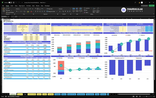
KPIs, forecasts, and cash flow at a glance.
Key assumptions and calculations driving revenue forecasts.
Funding sources, spending, and closing cash.
Cash break-even, payback, and ROIC.
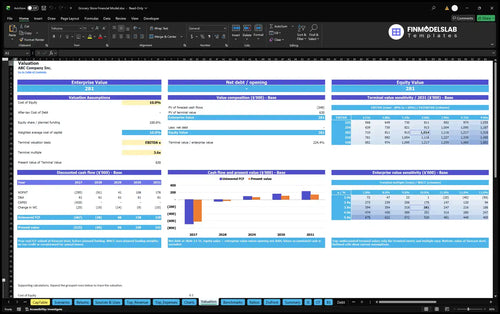
DCF valuation and sensitivity analysis.
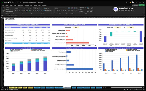
Largest costs and spending trends.
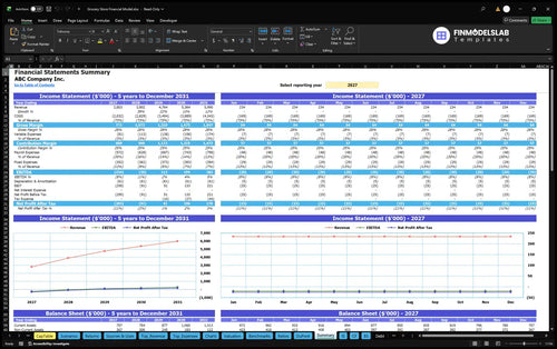
Annual and monthly financial performance.
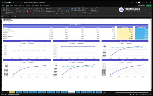
Compare margins and returns to benchmarks.

This template cut my build time down from days to a few hours, so I could focus on pricing and inventory instead of wrestling with formulas. That alone changed how fast we got our first forecast together.
I’m not deep into modeling, and this made the numbers easy to follow without feeling technical. I finished the projections and shared them with my partner the same afternoon.
Starting from zero always stalls me, but this gave me a clear place to begin. I had a working grocery store forecast in one sitting, which made the next planning call much easier.