

Revenue & Calc
Set expected monthly closings, frontage shares, finished-lot prices and launch timing. Revenue organizes these drivers; Calc translates them into monthly category volumes and revenue.


The Land Development Financial Model is an Excel template for projecting finished residential lot sales, operating expenses and EBITDA over 2026–2030. Its illustrative case follows a small developer that owns land in exurban Dallas-Fort Worth, Texas, commissions roads, drainage and utilities, then sells completed lots to homebuilders.
The case starts sales on January 31, 2026, with the first phase funded and prepared beforehand. Later phases replenish sold lots, but the operating forecast assumes a supplied development pipeline and does not schedule phase completion or inventory roll-forwards.
Edit the development assumptions and use the linked workbook schedules to examine their effect on lot revenue, operating earnings and funding.
Set expected monthly closings, frontage shares, finished-lot prices and launch timing. Revenue organizes these drivers; Calc translates them into monthly category volumes and revenue.
Adjust revenue-linked development and selling costs, monthly overhead and annual-average FTE. Separate contractor packages from employee base pay to understand which expenses scale with sales and which persist between closings.
Dashboard holds scenario and financing controls; CAPEX schedules asset purchases and depreciation. CapTable and Debt distinguish equity contributions from borrowing and its repayment obligations.
Standard workbook reports cover profitability, cash flow, financial position and a combined Summary. The supplied case establishes revenue, operating expenses and EBITDA; other report values depend on the completed financial model.
Expected homebuilder closings create one demand pool, allocated once across five frontage bands and multiplied by their finished-lot prices.
Monthly closings rise from 4 in 2026 to 8 in 2030, producing 48 to 96 expected annual sales. Prices and volume mix stay flat, so illustrated growth comes from additional closings without a parallel capacity control.
| Frontage | Share of lot volume | Price per lot |
|---|---|---|
| 40 feet | 20% | $70,000 |
| 50 feet | 30% | $85,000 |
| 60 feet | 25% | $100,000 |
| 70 feet | 15% | $125,000 |
| 80 feet | 10% | $160,000 |
The final 80-foot share is calculated after the first four bands; all volume shares total 100%.
Revenue Forecast translates closing volumes, frontage mix and finished-lot prices into sales by category, with launch timing preventing earlier revenue. Each lot is assigned once; fractional category volumes are planning expectations.
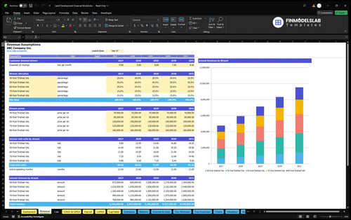
4 closings/month × 12 months × $99,250 weighted price/lot = $4,764,000 annual revenue.
Direct and variable costs scale with revenue, while overhead and fixed employee base pay are deducted separately to calculate EBITDA.
COGS and Operating Expenses separates revenue-linked development packages, selling expenses and monthly overhead. Direct costs total 74%: land allocation 32%, grading, roads and drainage 20%, utilities 14%, civil services 5%, and permits and connection fees 3%.
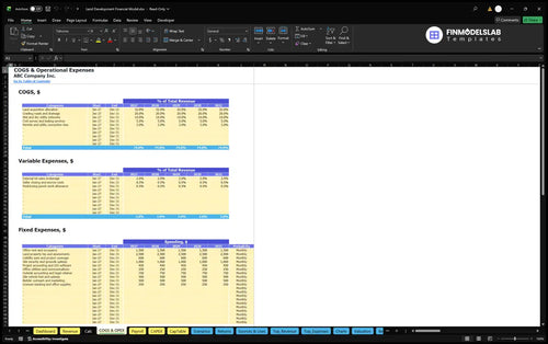
Variable costs total 3%: brokerage 2%, seller closing and escrow 0.5%, and punch work 0.5%. Fixed obligations total $99,600 each year, including $1,500 per month for office rent and occupancy, and remain payable throughout all twelve months.
Payroll Forecast by Staff Role models annual-average FTE and fixed base pay separately from contractor packages. Staffing increases from 2.5 to 3.5 FTE as the development manager and administrator roles expand; annual Payroll rises from $235,000 to $310,000.
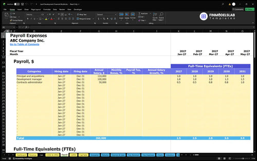
Annual base salaries per FTE are $110,000 for the principal, $100,000 for the development manager and $50,000 for the administrator. This example excludes employer taxes, benefits and personal taxes; outsourced civil packages are already included in COGS.
The estimated $4,480,449 owner contribution covers opening assets, separate startup cash, first-phase net working capital and a reserve for recurring outflows.
Capital Expenditure Plan schedules asset purchases and depreciation separately from operating expenses. The example starts with a $45,000 inspection vehicle, $6,000 in computers and office equipment, $3,000 in field equipment and $4,000 in furniture, totaling $58,000.
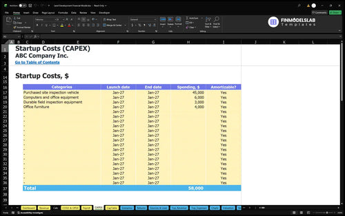
Separate opening cash covers refundable deposits, entity setup, builder sales materials, preopening management and project design fees. Working-capital controls are 0 receivable days, 14 payable days and 326 inventory days; these inputs do not constitute a phase-by-phase funding schedule.
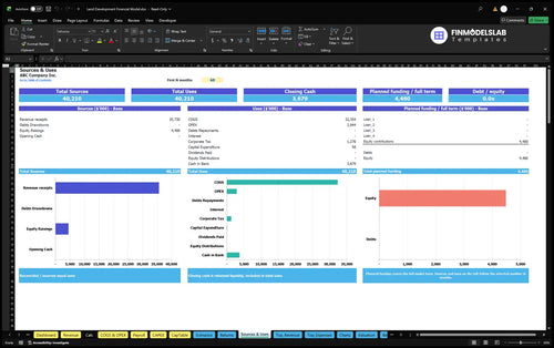
Sources and Uses of Funds reconciles cash sources, payments and retained cash over a selected forecast period. The opening estimate includes three months of recurring outflows and assumes zero committed outside funding; it does not establish peak project funding.
The illustrative case doubles annual revenue as monthly expected closings increase, while prices and frontage mix remain unchanged.
| Year | Revenue | Operating Expenses | EBITDA |
|---|---|---|---|
| 2026 | $4,764,000 | $4,002,880 | $761,120 |
| 2027 | $5,955,000 | $4,919,950 | $1,035,050 |
| 2028 | $7,146,000 | $5,849,520 | $1,296,480 |
| 2029 | $8,337,000 | $6,791,590 | $1,545,410 |
| 2030 | $9,528,000 | $7,746,160 | $1,781,840 |
Hypothetical planning outputs, not observed industry results; amounts are shown in whole US dollars.
EBITDA rises from $761,120 in 2026 to $1,781,840 in 2030, with margins of approximately 16.0% and 18.7%, respectively. These estimates deduct COGS, variable expenses, fixed obligations and Payroll, but do not establish after-tax profit or available cash.
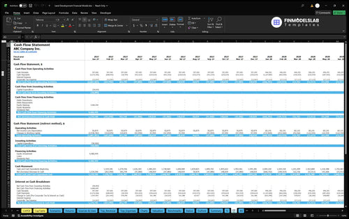
Cash Flow Forecast tracks operating, investing and financing movements, with an opening-to-closing cash reconciliation. Lot-sale cash arrives through escrow at title transfer in this case; review development payments and funding separately because an EBITDA surplus does not prove liquidity.
Returns separates operating cost coverage, cash break-even, investment recovery and annual return on invested capital.
Returns compares revenue with sales break-even requirements, tracks cash break-even and project payback, and calculates annual ROIC. Use these distinct measures to assess operating coverage, cash timing and invested capital after reviewing the underlying cash-flow inputs.
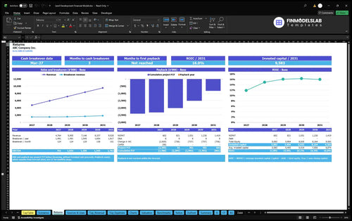
Sales break-even addresses revenue needed to cover operating costs; cash break-even addresses cash-flow timing. Investment payback measures recovery of invested cash, while annual ROIC relates operating returns to invested capital.
Dashboard Low, Base and High controls vary revenue, COGS, variable expenses, fixed expenses and Payroll. Debt controls allow four facilities with repayment structures and terms; no loan draw, interest rate, payback date or ROIC result is established by this brief.
Use this template for a small owned-inventory residential lot developer selling finished lots directly to homebuilders.
The case assumes completed roads, drainage and utilities at sale, no customer credit and no future development obligations. Evaluate expected closings, price mix, cost ratios and staffing against your own pipeline before using the financial projections.
Estimated inputs are planning selections, not independently verified local market benchmarks. Projects needing detailed construction milestones, land inventory movements or peak funding tests require additional schedules.
These answers explain the editable assumptions, operating scope and limits of the illustrated results.
Edit expected closings, frontage mix, prices, sales launch timing, cost percentages, overhead, staffing, working-capital days, asset purchases and funding controls to reflect your own assumptions.
The illustrated operating case assumes a supplied development pipeline; it does not schedule phase completion or detailed inventory roll-forwards.
No; the lot prices, cost ratios and funding amounts are estimated planning inputs, and the companion references do not independently verify these selections.
No; fractional frontage-category volumes express expected allocations across the sales pool, while each completed transaction transfers an individual lot.
No; EBITDA excludes investment and financing cash movements, and the initial owner-funding reserve does not test peak funding needs across development phases.
The standard Returns report calculates these measures from cash flows and invested capital, but the supplied illustrative case provides no verified payback date or ROIC value.
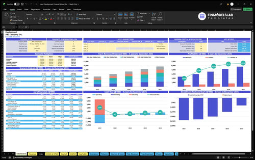
KPIs, forecasts, and cash flow at a glance.
Key assumptions and calculations driving revenue forecasts.
Funding sources, spending, and closing cash.
Cash break-even, payback, and ROIC.
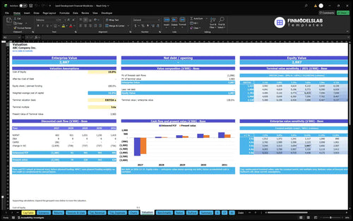
DCF valuation and sensitivity analysis.
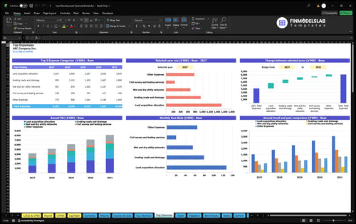
Largest costs and spending trends.
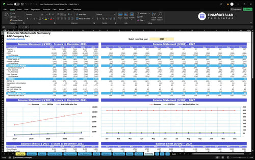
Annual and monthly financial performance.
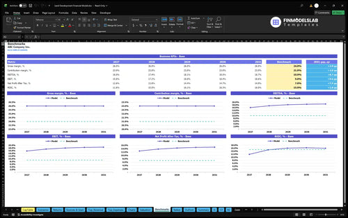
Compare margins and returns to benchmarks.

This model made margins and break-even easy to see instead of buried in formulas. I cut my review time by a few hours and could explain profitability to our partner in one meeting.
Low, base, and high cases were simple to switch between, so I stopped rebuilding the same assumptions over and over. It saved me an afternoon and made our planning conversation much cleaner.
I liked having the statements and charts together instead of hunting through separate files. It cleaned up our reporting package fast, and I sent the full update to the team the same day.