

Revenue & Calc
Edit monthly visits, purchase conversion, units per transaction, seasonal multipliers, category shares, and net prices. Monthly calculations feed the six record-sales lines into projected revenue.


The Record Store Financial Model is an Excel planning template for an independent 1,200-square-foot U.S. vinyl shop operating six days a week. It builds illustrative 2026–2030 projections from store visits, buying conversion, items per purchase, category mix, realized prices, and seasonal demand.
The example covers six new and used record categories sold in-store, with payment collected at purchase and stock bought without supplier credit. It excludes e-commerce, consignment, paid events, equipment resale, and customer credit sales; forecast amounts are in U.S. dollars.
The linked worksheets turn record-store operating inputs into monthly calculations, forecast reports, and funding and investment analysis.
Edit monthly visits, purchase conversion, units per transaction, seasonal multipliers, category shares, and net prices. Monthly calculations feed the six record-sales lines into projected revenue.
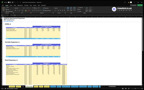
Plan vinyl purchases, freight, shrink, processing fees, marketing, occupancy, and store overhead separately from the owner-manager and record associates’ salaries.
Schedule opening fixtures and equipment, record owner contributions, and review how investment, working capital, and operating payments affect planned cash uses.
Review Dashboard, Income Statement, Cash Flow, Balance Sheet, Scenarios, Returns, and Checks for connected financial reporting and input consistency.
The record store’s revenue forecast follows purchasing demand rather than an independent floor-space or checkout-capacity limit.
Monthly sales volume equals store visits multiplied by purchasing conversion, items per purchasing visit, and that month’s seasonal factor. In the 2026 illustrative case, 2,200 visits, 38% conversion, and 1.5 items per purchase imply 1,254 items before seasonality.
The item mix allocates 40% to new standard LPs, 10% to new deluxe LPs, 25% to used regular LPs, 12% to used collectibles, 8% to seven-inch singles, and 5% to bargain LPs. Each category has its own net selling price.
The Revenue Forecast connects store traffic, purchasing behavior, unit mix, and prices to annual sales by record category. The Calc sheet applies the repeating seasonal profile to the monthly forecast.
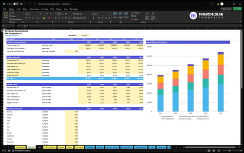
2,200 visits × 38% conversion × 1.5 items × $26.28 weighted net price ≈ $32,955 sales before seasonality.
April and November each use a 1.30 seasonal multiplier; December uses 1.40. Monthly visit assumptions increase to 3,000 by 2030, while conversion rises to 42%. All are editable estimates, not independently verified industry averages.
The financial model separates merchandise-related costs, revenue-linked expenses, fixed store overhead, and salaries so each cost is counted once.
Estimated direct costs equal 55.5% of sales: 53% inventory purchases, 1.5% inbound freight, and 1% damage or shrink. Variable expenses add 5.3% of sales for payment processing, ongoing marketing, and checkout supplies.
The COGS and Operating Expenses forecast keeps merchandise costs and sales-linked charges separate from monthly store overhead. Fixed inputs cover rent, shared-area costs, utilities, insurance, software, accounting, cleaning, maintenance, and related operating needs.
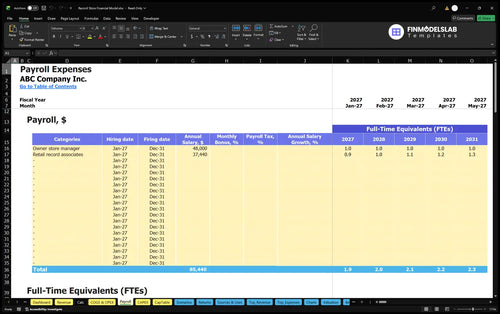
The owner-manager is budgeted at one full-time equivalent and $48,000 annual base pay. Record associates increase from 0.9 average FTE in 2026 to 1.3 in 2030, using $37,440 annual base pay per FTE.
The Payroll Forecast plans staffing by role, annual-average FTE, base compensation, and monthly timing. In the illustrative operating case, total annual base payroll increases from $81,696 in 2026 to $96,672 in 2030.
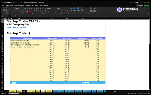
Opening investment is modeled separately from the store’s recurring operating earnings, with inventory needs controlled by working-capital assumptions.
The opening asset budget totals $37,000: $18,000 for leasehold improvements, $10,000 for record bins and shelving, $5,000 for POS and listening equipment, and $4,000 for signage and security. A refundable deposit and opening campaign and permit payments are separate cash items.
The Capital Expenditure Plan schedules store build-out, fixtures, electronics, and security purchases and distinguishes depreciable assets from other spending. These asset outlays are not the same as the annual EBITDA expense categories.
The example sets 115 inventory days, zero receivable days, and zero payable days, consistent with cash-at-sale customers and prepaid or acquisition-time stock purchases. Initial owner funding is estimated at $206,932, including opening cash needs and three months of recurring outflows.
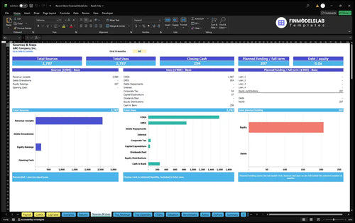
The Sources and Uses of Funds report helps reconcile planned equity or debt sources against inventory, opening investment, operating payments, and retained cash. It makes financing allocation review distinct from the income statement’s earnings calculation.
The selected example projects higher store sales and EBITDA from 2026 through 2030 under its stated demand and expense assumptions.
| Year | Revenue | Operating Expenses | EBITDA |
|---|---|---|---|
| 2026 | $395,461 | $375,897 | $19,565 |
| 2027 | $451,621 | $412,186 | $39,434 |
| 2028 | $511,844 | $453,986 | $57,858 |
| 2029 | $576,321 | $498,413 | $77,908 |
| 2030 | $645,094 | $545,493 | $99,601 |
Illustrative projections, not historical results or industry averages. Figures are rounded to whole dollars; displayed arithmetic may differ slightly.
Operating expenses include COGS, variable operating expenses, fixed overhead, and Payroll. For 2026, the estimated breakdown is $219,481 of direct costs, $20,959 of variable expenses, $53,760 of fixed expenses, and $81,696 of payroll.
EBITDA is operating earnings before interest, tax, depreciation, and amortization. The table does not establish net profit, free cash flow, financing repayment capacity, or a positive cash balance.
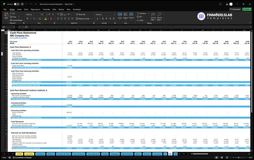
The Cash Flow Forecast tracks operating receipts and payments together with capital expenditures, financing movements, and cash reconciliations. This is where an owner evaluates liquidity effects that the operating EBITDA forecast cannot show on its own.
The model provides different views of operating break-even, actual cash recovery, investment returns, and the sensitivity of record-store assumptions.
The Returns analysis separates sales break-even, cash break-even timing, investment payback, and annual return on invested capital. A store can reach operating break-even without recovering its upfront investment or producing sufficient cash at every date.

Use sales break-even to compare the required sales level with modeled traffic and basket size. Use payback to examine cumulative project cash recovery, and ROIC to evaluate invested-capital returns; none can be deduced from EBITDA alone.
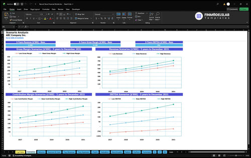
The Financial Scenario Analysis compares Low, Base, and High cases using adjustable multipliers for revenue, direct costs, variable expenses, fixed overhead, and payroll. It helps examine how weaker conversion or a tougher cost structure changes projected operating margins.
The Dashboard also includes debt-facility inputs, while the financial reports cover cash flow and balance-sheet consequences if financing is entered. No specific loan, project payback date, ROIC, or valuation amount is asserted for this example.
The template suits an owner evaluating a single neighborhood shop with direct in-store vinyl sales and a straightforward purchasing model.
It can support lease discussions, category assortment planning, staffing choices, inventory purchasing, and funding conversations. A store with online shipping, consignment inventory, events, or wholesale credit should revise the scope instead of treating this case as a validated fit.
These answers clarify which store operations are modeled and which financial results still require case-specific review.
Yes. Revenue inputs include monthly visits, purchase conversion, units per visit, seasonality, item mix, and annual prices by vinyl category.
No. The documented scenario models in-store transactions only, without e-commerce fulfillment, shipping, or marketplace fees.
Yes. Used collectible LPs, used regular LPs, and bargain LPs have separate sales shares and net prices.
The illustrative assumptions use 115 inventory days, no accounts receivable period, and no supplier payable period. Inventory is acquired without credit.
Yes. One owner-manager FTE receives $48,000 in annual base pay, separate from the associates’ salary budget.
No. EBITDA excludes depreciation, interest, and tax, and it does not represent cash flow or recovered startup investment.
No. The estimated opening contribution is a planning input; cash balances and funding needs require a separate review of the model’s cash flow and balance sheet.
Yes. Dashboard controls and Scenarios compare Low, Base, and High cases by changing revenue and operating-cost multipliers.
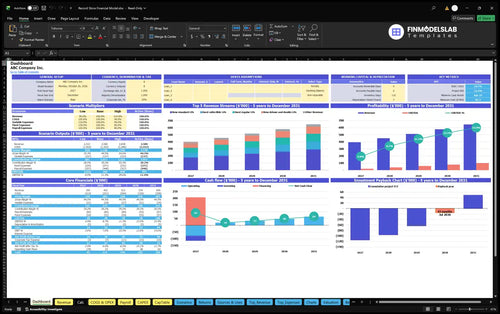
KPIs, forecasts, and cash flow at a glance.
Key assumptions and calculations driving revenue forecasts.
Funding sources, spending, and closing cash.
Cash break-even, payback, and ROIC.
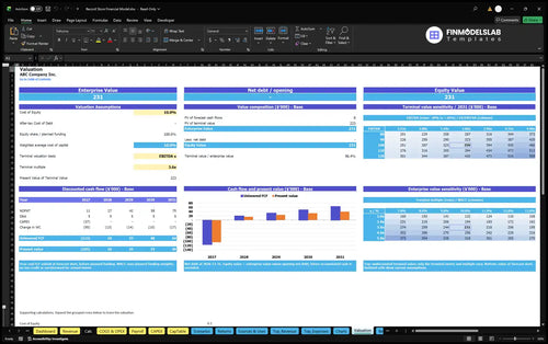
DCF valuation and sensitivity analysis.
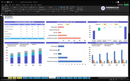
Largest costs and spending trends.
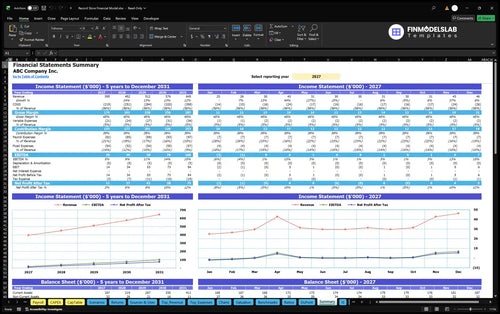
Annual and monthly financial performance.
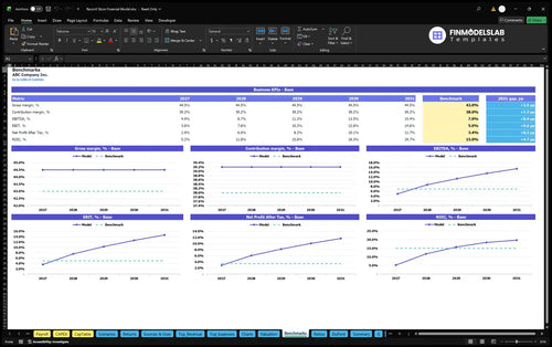
Compare margins and returns to benchmarks.

The pricing, cost, and growth tabs finally felt organized instead of scattered, so I could build a cleaner forecast in one sitting. It cut my assumption review from half a day to about an hour.
I’m not strong in Excel, and this template made the modeling side feel much less technical. I was able to update the numbers myself and send the file to my partner the same day.
Before this, my statements and charts were spread across different files. Now everything is in one model, and I had investor-ready reporting ready for a meeting without piecing it together last minute.