

Revenue and Calc
Change monthly visits, purchase conversion, pairs per transaction, six category prices and shares, and the calendar-month seasonality profile. Calc translates these drivers into monthly footwear sales.


The Shoe Store Financial Model is an Excel financial projection template for an independent, 1,800-square-foot suburban U.S. footwear retailer. It converts customer visits, buying conversion, pairs purchased, category mix, and realized shoe prices into monthly sales and a five-year operating forecast.
The illustrated business sells footwear in-store six days per week, with no online channel or customer credit. Its 2026–2030 assumptions are editable planning estimates, not observed store results, market averages, or guaranteed performance.
The workbook links store-specific operating assumptions to monthly calculations, financial statements, and decision reports.
Change monthly visits, purchase conversion, pairs per transaction, six category prices and shares, and the calendar-month seasonality profile. Calc translates these drivers into monthly footwear sales.
Plan shoe purchase costs, freight, shrink, processing, local marketing, rent, and staff compensation separately. Role-level staffing and fixed pay feed the expense calculations without double-counting wages.
Use centralized dates, working-capital settings, Low/Base/High scenario multipliers, and optional debt controls. CAPEX, CapTable, and Debt support startup investments, equity, and financing schedules.
Review Income Statement, Cash Flow, Balance Sheet, Summary, Sources & Uses, Scenarios, Returns, Valuation, Ratios, and checks. These reporting functions are available without implying case-specific figures not shown here.
Sales are driven by store visits multiplied by purchase conversion, pairs per buying visit, seasonal demand, and category-specific net prices.
In the illustrated case, monthly visits increase from 2,200 in 2026 to 3,100 in 2030, while purchasing conversion rises from 26% to 30%. Each purchasing visit averages 1.1 pairs; the model does not add a separate, competing sales-capacity forecast.
Pairs are allocated across women’s casual (23%), men’s casual (20%), adult athletic (22%), children’s (15%), work boots (10%), and dress shoes/sandals (10%). Each group uses its own annual net selling price, after sales tax, markdowns, and expected returns.
The Revenue Forecast shows how store traffic, conversion, pairs per purchase, and six product-group prices determine unit volumes and sales. Its inputs connect to the Calc worksheet’s monthly forecast, so changing the mix or price changes projected revenue.
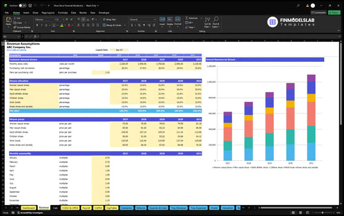
2,200 visits/month × 26% conversion × 1.1 pairs × $82.35 weighted price × 12.0 annual seasonality units ≈ $621,775 revenue.
The seasonal profile assigns August a 1.40 multiplier compared with 0.75 in both January and February. November and December carry 1.15 and 1.20; the twelve factors total 12.0, preserving the annual average while moving sales between months.
The model separates footwear acquisition costs, revenue-linked operating expenses, monthly fixed overhead, and fixed-base payroll.
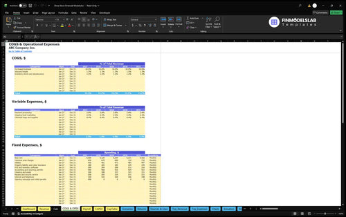
Direct costs total 54.7% of sales in the example: 52% purchased shoes, 1.5% inbound freight, and 1.2% shrink or obsolescence. Variable expenses add 5.7% for payment processing, ongoing local marketing, and checkout supplies.
The remaining expense plan includes base rent, common-area charges, utilities, insurance, software, accounting, cleaning, repairs, security, and communications. Illustrative monthly base rent is $4,000 in 2026 and $4,502 in 2030.
The COGS and Operating Expenses forecast separates percentage-based shoe procurement and transaction costs from fixed monthly overhead. Compare the operating cost structure with changing sales before deciding whether pricing, marketing, or purchasing assumptions need revision.
| Cost group | Calculation basis | Annual amount |
|---|---|---|
| COGS | 54.7% of sales | $340,111 |
| Variable | 5.7% of sales | $35,441 |
| Fixed | Monthly expense plan | $82,560 |
| Payroll | Fixed salary plan | $110,160 |
The four expense groups total approximately $568,272; payroll is not also charged within COGS or other operating expenses.
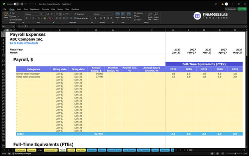
The Payroll Forecast tracks one full-time owner-manager earning $54,000 annually, plus sales associates averaging 1.5 FTE in 2026 and 2.0 FTE in 2030 at $37,440 per annual FTE. Salary changes and staffing decisions feed personnel costs.
Startup equipment, opening cash requirements, working-capital assumptions, and owner funding are distinct from recurring operating earnings.
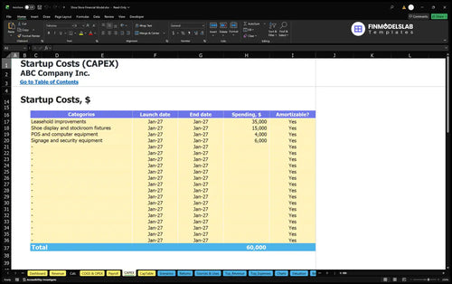
The example budgets $35,000 for leasehold improvements, $15,000 for footwear displays and stockroom fixtures, $4,000 for POS and computers, and $6,000 for signage and security. These planned asset purchases total $60,000, before other opening cash needs.
The Capital Expenditure Plan schedules the store fit-out, fixtures, systems, and security assets, with depreciation and asset balances handled in the supporting workbook schedules. Capital purchases are not the same as annual footwear procurement expenses.
The working-capital inputs are 86 inventory days, 29 accounts-payable days, and zero receivable days because customers do not buy on credit. Stock commitments and supplier payment timing therefore matter even when the income statement shows positive EBITDA.
Illustrative initial owner funding is $266,817, based on startup assets, a refundable lease deposit, opening costs, net working capital, and three months of recurring first-year outflows. The reserve excludes the one-time opening campaign and initial permits.
The Sources and Uses of Funds report reconciles equity, any modeled borrowing, operating receipts, investment, and payments over the selected period. It helps distinguish the proposed owner contribution from earned revenue and compare funding with planned cash allocation.

The illustrated case reports annual footwear revenue, total operating expenses, and EBITDA from 2026 through 2030.
| Year | Revenue | Operating expenses | EBITDA |
|---|---|---|---|
| 2026 | $621,775 | $568,272 | $53,503 |
| 2027 | $748,413 | $645,887 | $102,527 |
| 2028 | $870,818 | $727,678 | $143,140 |
| 2029 | $986,875 | $805,699 | $181,176 |
| 2030 | $1,094,253 | $876,672 | $217,581 |
Planning scenario, not historical performance. Dollar amounts are rounded independently, so displayed differences can vary by $1.
In this case, annual EBITDA rises from $53,503 in 2026 to $217,581 in 2030 as visit volume, conversion, and net prices increase. That is operating earnings before depreciation, interest, and taxes—not net profit, free cash flow, or money available for distribution.
The Income Statement, Balance Sheet, and Cash Flow schedules extend the workbook’s reporting beyond these illustrative EBITDA outputs. No case-specific net income, debt balances, or closing cash totals are asserted by this example.
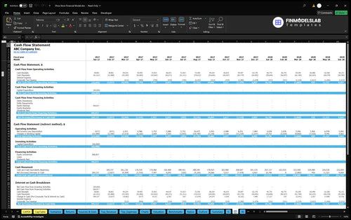
The Cash Flow Forecast follows operating receipts and payments, startup investment, equity funding, and any configured debt activity to projected cash balances. Use it to test whether inventory purchases and opening expenses create liquidity pressure despite positive operating EBITDA.
The Returns and scenario reports address different questions about operating coverage, recovery of invested cash, and investment performance.
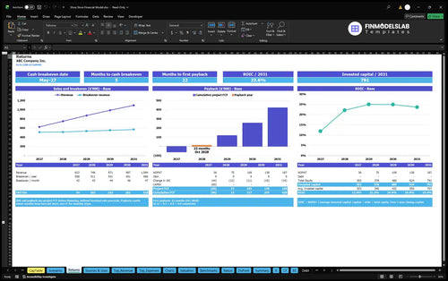
The Returns analysis distinguishes sales break-even from cash break-even timing, cumulative investment payback, and annual return on invested capital. These measures require their own cash flows and invested-capital inputs; the example EBITDA table cannot establish payback or ROIC.
Use Dashboard scenario controls to compare Low, Base, and High cases by changing revenue, direct costs, variable expenses, fixed expenses, and payroll multipliers. Scenarios then shows how changed sales and margins affect projected EBITDA rather than treating one forecast as certain.
Optional Dashboard debt controls provide four facility rows with borrowing dates, terms, interest-only periods, rates, and repayment structures. The Valuation, Ratios, and Benchmarks reports offer additional analyses, but this page does not claim a specific valuation, IRR, loan approval, or investment return.
This model fits owners and analysts planning an independent physical shoe store with category-level sales and meaningful inventory needs.
It supports decisions about store traffic targets, footwear assortment, associate coverage, rent affordability, opening investment, and potential funding gaps. Replace the illustrative inputs with your own local demand, realized prices, supplier terms, payroll burden, and lease economics before using the projections to make decisions.
Quick answers about model inputs, forecast scope, financing, and the reported results.
Yes. Edit visits, buying conversion, pairs per purchasing visit, and seasonality in Revenue to recalculate monthly footwear demand and sales.
Yes. Women’s casual, men’s casual, adult athletic, children’s, work boots, and dress shoes/sandals have distinct revenue shares and annual net prices.
No. The example assumes in-store footwear sales only, six days per week, without ecommerce revenue or customer credit.
Yes. The example uses 86 inventory days, 29 payable days, and zero receivable days; these are editable working-capital inputs.
No. EBITDA precedes depreciation, financing costs, and taxes. The full workbook includes financial statements, but the displayed example only supplies operating results through EBITDA.
No. The owner-manager and sales-associate base salaries sit in Payroll, separate from purchased shoes, freight, shrink, and other expenses.
Yes. Dashboard debt controls, Sources & Uses, Cash Flow, and Returns help evaluate financing, break-even, payback, and ROIC after suitable case inputs are entered.
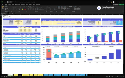
KPIs, forecasts, and cash flow at a glance.
Key assumptions and calculations driving revenue forecasts.
Funding sources, spending, and closing cash.
Cash break-even, payback, and ROIC.
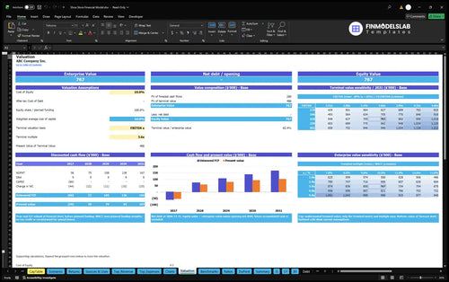
DCF valuation and sensitivity analysis.
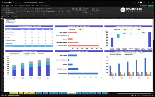
Largest costs and spending trends.
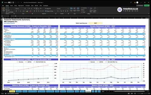
Annual and monthly financial performance.
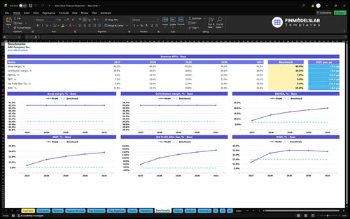
Compare margins and returns to benchmarks.

This template made the required outputs and structure much easier to understand, so I could build a clean investor pack without second-guessing the layout. It saved me a full day of guessing what to include.
I stopped worrying about one broken cell throwing off the whole model. The formulas were already set up cleanly, so I spent less time checking links and more time finishing the forecast.
The pricing, cost, and growth inputs were organized in a way that finally made sense. I got through my first planning pass in about two hours and had a clearer story for the numbers.